

Calculating Collatz
Part One: The original and three variations

Playing around with the Collatz conjecture over the summer has been quite a lot of fun, and I’m finally getting close to the point where I shall be disclosing some of my findings. I’m happy to report that I’ve “proved” the conjecture at least four or five times. Alas, three or four of those '“proofs” turned out to not be proofs at all.
As for the veracity of the fourth or fifth? We shall see. That won’t be for me to decide, unless I debunk them myself, which I’ve been doing my best to do prior to publishing. Be all that as it may, I have enough material now on the topic for many posts to come, which, if nothing else, can offer pedagogical value for the learning of mathematics.
So, to help those interested in following along, or better yet, delving into the problem further of their own accord, I’m going to begin with an illustration of three variations for calculating Collatz aside from the Collatz function itself, all three variations essentially being “shortcuts” of the original.
The Collatz Function
As discussed in previous posts here and here, the Collatz function itself is as follows:
It will be helpful for those following along to start thinking more in terms of modular arithmetic, which has been one of the greatest innovations for studying structures and relationships amongst numbers in the history of number theory.
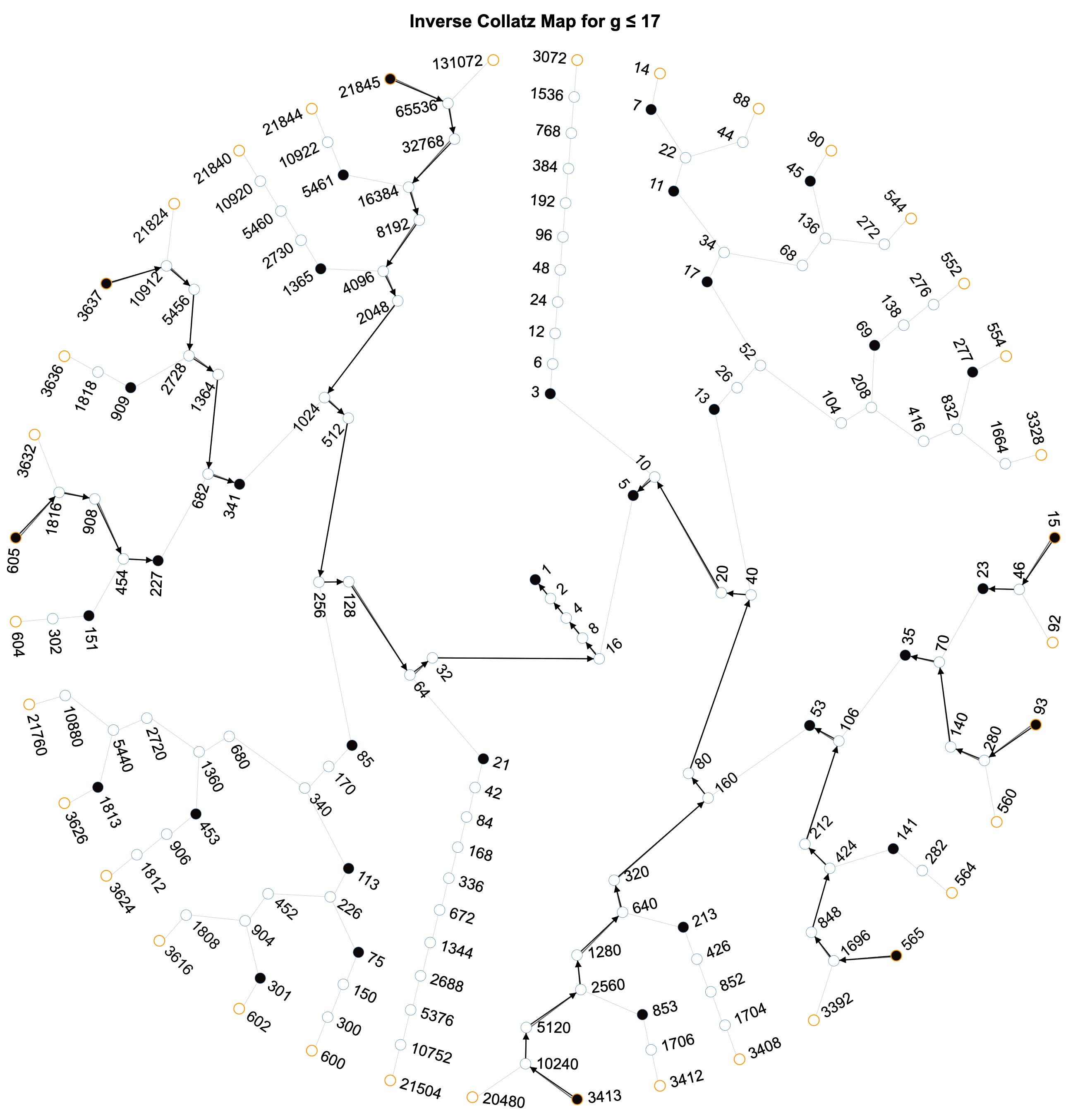
For illustrative purposes, using the Inverse Collatz Map, a single application of C(n) on values with the same total stopping times (the number of iterations of C(n) where the starting values terminate at 1, in this case, all the values which share a total stopping time of 17 look like this:

Note above that odd values are indicated by black circles; even values by white circles. Light line segments illustrate the trajectories that numbers take in converging toward 1 as the Collatz function is iteratively applied.
This classic Collatz function, while largely having been superseded by the variations that follow for computational and analytical reasons, is both historically canonical and pedagogically ideal for introducing the conjecture to students and other practitioners of mathematics. It reveals the function’s “zig-zag,” “hailstone” structure and is the natural approach for reporting total stopping times and classical peaks.
Here is the very “zig-zaggy” looking “hailstone” trajectory for C(n) when n = 27:
The Terras Function
In 1976, exploiting the fact that, for odd n, 3n + 1 is always an even number, Riho Terras introduced the following variation of the Collatz function:
When n is odd, this formulation combines an odd-step and an even-step of the standard Collatz function into a single iteration. The T(n) function ensures that at each iteration the iterative sequence is at least partially brought “back down” after an odd step, instead of skyrocketing by a factor of 3 with no immediate reduction. This made it easier for Terras to analyse the balance between multiplication by 3 and division by 2 over the course of a number’s Collatz trajectory.1
The following diagram illustrates the effect of Terras’s function on odd values (the black circles). Treatment of even numbers remains exactly the same as for the original Collatz function C(n) above so their trajectories remain the same as above and are not indicated here to avoid clutter and to help better focus on the behaviour of odd n:

The significance of Terras’s modification is it enabled him to analyse the behaviour of the Collatz function (approximately, that is, by ignoring the small +1 increments) in terms of the ratio between the number of tripling steps and the number of halving steps in a positive integer’s Collatz trajectory. This clever formulation allowed Terras to translate the stopping time problem (viz., the number of iterations to convergence to 1), into questions about parity sequences of odd/even steps and, further, to eventually estimate how stopping times are distributed.2
The Syracuse Function
The Collatz conjecture dates back to 1937, and over time acquired many names, such as the “Syracuse problem,” a term proposed by Helmut Hasse in the 1950s during a visit to Syracuse University. However, the function known as the Syracuse function was first explicitly formulated in the late 1970s by Herbert Möller.3 It was quickly adopted by those seeking more analytically convenient formulations of the Collatz function, which has enabled taking Terras’s ideas a few steps further.
The Syracuse function, S(n),4 is an accelerated form of both the Collatz and Terras functions, in that for odd n, 3n + 1 is divided by 2 to the power of the 2-adic valuation of 3n + 1 (viz., 2 to the maximal power of 2 that divides 3n + 1). Symbolically:
Möller’s formulation rolls all even steps that follow an odd step into one combined operation. That is, starting from an odd number, one performs the 3n + 1 step and then immediately divides by 2 as many times as possible. Computationally, this division is easily done with 3n + 1 encoded in binary, by simply counting trailing zeroes, then right-shifting the bit-string by that amount. In doing so, one jumps directly to the next odd number in the trajectory, as illustrated below:
The Syracuse function is currently considered the modern analytic baseline for investigating the Collatz conjecture. It reduces the conjecture to the odd integers, because every even run is uniquely determined (see Figures 4 & 5, below). Proving convergence for S(n) on the odds suffices to prove the full Collatz conjecture.

But what about the even numbers? It is implicit when using S(n) to assume that if one starts with an even number, n, that one simply iteratively divides n by 2 until an odd number is reached. So, why not just make this condition explicit?
The R(n) function
Let’s do that then, if only for pedagogical reasons, by introducing the R(n) function. This variation simply divides even n by its 2_adic valuation as well. Note that this tweak of S(n) only pertains to starting with even n, as after the first iteration, all subsequent values in n’s trajectory will be odd values.
I have found this trivial variation of the Syracuse function helpful in my own investigations of the Collatz conjecture, in that it renders some important aspects of the Collatz structure and dynamics more transparent. First and foremost, and one of my earliest and delightful “aha moments” in my investigations, was the realization that the cardinality of the set of all numbers with the same stopping time, g, was equivalent to the cardinality of the set of all odd numbers with total stopping times less than or equal to g.5 Figure 5, as with Figure 4 above, offers a more radial6 representation, and a more intuitive way of seeing this structure:

As I’ve indicated previously, the Inverse Collatz Map is an excellent, and a very seductive,7 way for exploring the Collatz conjecture. For instance, I have found it quite helpful, for reasons I will divulge in due course, to focus on the sets of even predecessors of odd numbers, which I have come to refer to as dyadic rays:

Concluding Remarks
It is important to note that all the above formulations of the Collatz conjecture are equivalent. Proving the conjecture true using one proves the conjecture for them all. However, as I hope is more evident now, certain properties are easier to express in one form or the other. The Terras function, or map, was key to proving almost all numbers eventually go down (finite total stopping times), and the Syracuse map has been key to the latest deep results (viz., Tao’s theorem).8
The standard map is most intuitive and is the one to which undecidability results apply (Conway showed a generalization of that form is undecidable). The Syracuse function has no known cycles other than 1, just as the standard function has no known cycles other than 4-2-1; if a non-trivial cycle exists in one model, then it must exist in the others. So, behaviourally, with regard to the structure and dynamics of the Collatz conjecture, these variations don’t change what the problem is, but rather, simply repackages it.
I’ll leave the reader with this numerical comparison of the last few iterations of C, T, and S for n = 27, including full displays of the trajectories for all three:9

Collatz trajectories are also referred to as orbits. I prefer using the former.
Terras, Riho. “A stopping time problem on the positive integers.” Acta Arith, 30.3 (1976): 241-252. http://matwbn.icm.edu.pl/ksiazki/aa/aa30/aa3034.pdf
Möller, Herbert. “Über hasses verallgemeinerung des syracuse-algorithmus (kakutanis problem).” Acta Arith, 34 (1978): 219-226. matwbn.icm.edu.pl/ksiazki/aa/aa34/aa3435.pdf
The Syracuse function is often written as Syr(n). I prefer the simplicity of S(n), and for a few other reasons that will become more apparent in subsequent posts.
I later discovered, not surprisingly, that I wasn’t the first to have this realization.
As I haven’t yet come across a radial representation of the Inverse Collatz Map, and if this is indeed the first time such a representation has been published, I suppose I may be able to claim this modest visual innovation as an original contribution in this regard.
Seductive, in that it is so easy to assume that uncovering various structures and dynamics of the Inverse Collatz Map (ICM) can entail a proof of the Collatz conjecture, when in fact, one is implicitly assuming all numbers in the ICM converge, because they converge.
Tao, Terence. “Almost all orbits of the Collatz map attain almost bounded values.” Forum of Mathematics, Pi. Vol. 10 Cambridge University Press, 2022.
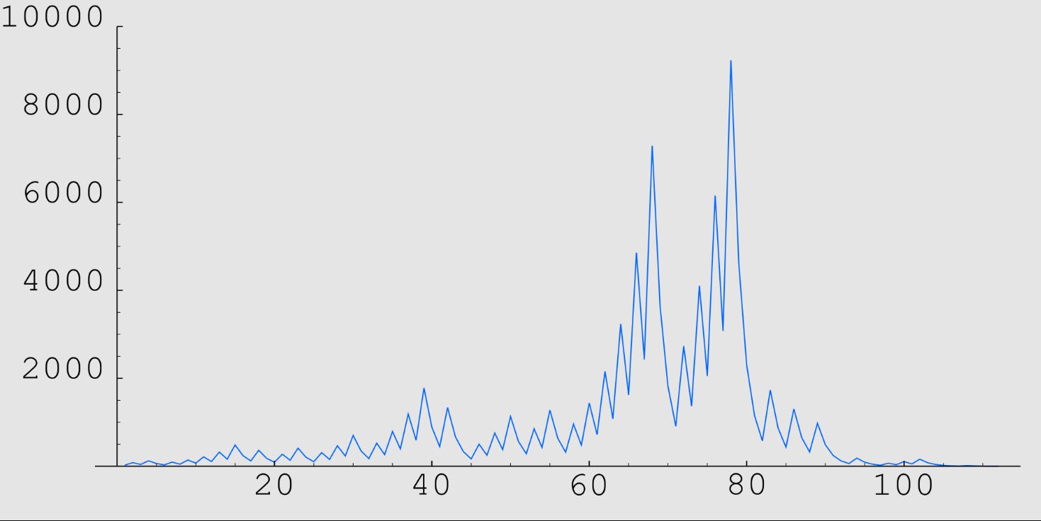
Note: the y-axis of the displays are iterate values in “bits(n)” (essentially log_2(n)). Otherwise, for large excursions, the display becomes visually useless quickly.