

The Inverse Collatz Map
This one's for you, Bert!

When I first came across the ICM after having recently encountered the Collatz Conjecture (see my post few weeks ago here), I was immediately enthralled.1
The ICM provided me with a completely new perspective on the Collatz function:
I had been under the impression that the Collatz function, T(n), if true, produced a plethora of excursions (also referred to as trajectories, or orbits) through a finite, up and down (“hailstone”), sequence of numbers and that for all n, such that n ≥ 1 would find its way to 1 in a finite number of iterations, commonly referred to as the total stopping time, at which point the iterations loop infinitely 1 —> 4 —> 2 —> 1
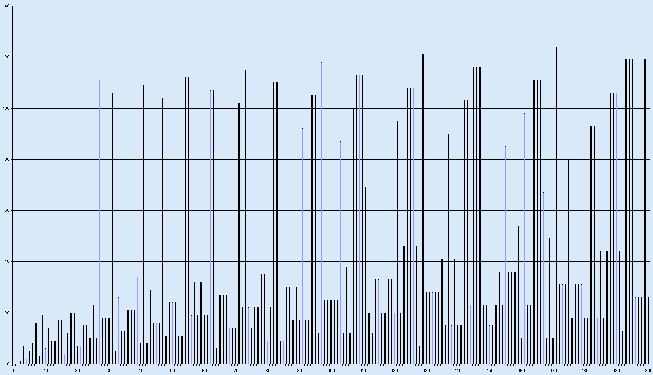
Looking at the total stopping times for C(n) for the first couple of hundred values of n one might quite reasonably think that the function behaves rather randomly:
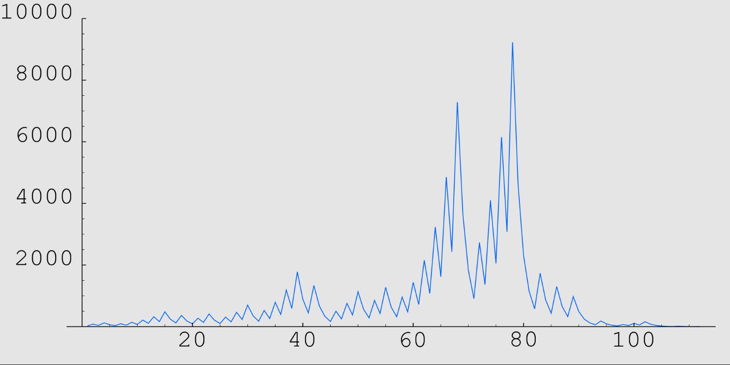
Here is the very random looking “hailstone” trajectory for C(n) with n = 27:
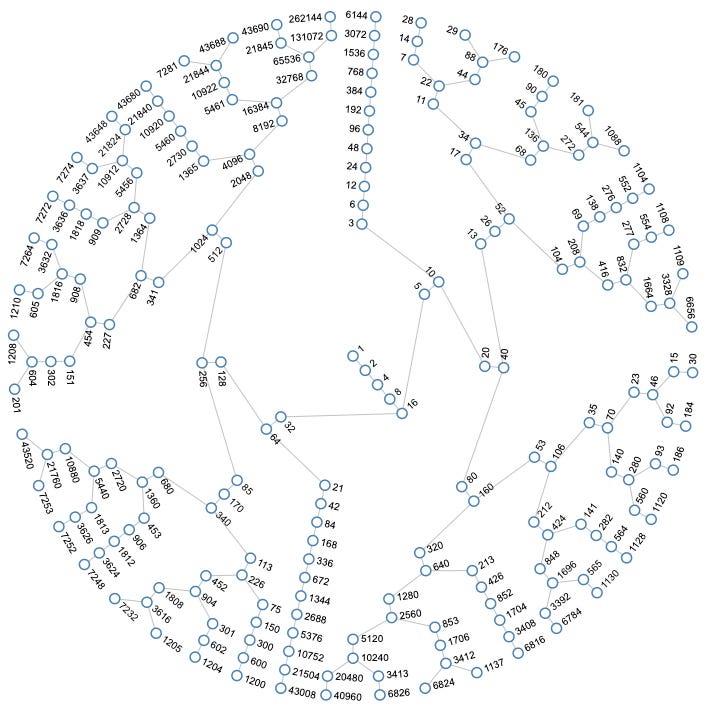
The longer I gazed at the ICM (in a trance state well known to mathematicians), the more my preconceptions regarding the randomness of the Collatz Function dissolved, until they seductively disappeared completely. There was structure within the ICM. Lots of it. The more deeply I looked, the more that structure revealed itself to me:
Yes, I must admit, I was seduced. Seduced into thinking therein must lie the elusive solution to this longstanding conjecture. The siren song of a proof beguiled me. Unlike Odysseus, unbound to any mast, I dove right in… captivated.
The first thing I noticed was how the ICM revealed different families of numbers with each new generation. It came quite naturally to think about the numbers in the same generational level in familial terms, along with their ancestors and descendants. The second thing I noticed was the clustered distribution of numbers in each generation. There wasn’t much randomness I could see in that, and having expected such, I was shocked. Take the members of generational level 18:2
Cluster 0: 262144 (= 2 to the 18th power, btw)
Cluster 1: 43690, 43688, 43680, 43648, 43520, 43008, 40960
Cluster 2: 7281, 7274, 7272, 7264, 7253, 7248, 7232, 6826, 6824, 6816, 6784, 6656
Cluster 3: 1210, 1205, 1204, 1200, 1137, 1130, 1128, 1120, 1109, 1108, 1104, 1088
Cluster 4: 201, 186, 184, 181, 180, 176
Cluster 5: 30, 29, 28
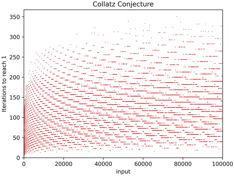
Does anything about that structure look “random” to you? It sure didn’t to me. More recently I came across this graph, which does a pretty good job of revealing the ICM distributional structure as the generational levels increase:
Anyone with experience in studying sequences of numbers knows that further insights can often be gained by looking at differences between numbers within those sequences. I invite the reader to do that with the clusters above. Notice anything?
(Hint: powers of 2, but we’ll return to that later… stay tuned).
In terms of structure, what is most visually notable about the ICM is the “branching,” or lack thereof. Indeed, branching appears to have quite a multitude of “stems” of two numbers, e.g., (5, 10), (32, 64), etc., a lesser multitude of stems of three numbers, e.g., (13, 26, 52), (85, 170, 340), etc., a few stems that appear to continue indefinitely, e.g., (3, 6, 12…), (21, 42, 84…), etc., and one original stem of five numbers (1, 2, 4, 8, 16), which as it turns out, is just a stem of three numbers concatenated with a stem of two numbers.
The immediate question that arises, is what can account for these differences? Why, for instance, does 16 branch? Does it have anything in common with other branch points? If so, what might that be? It would seem that any attempt to tease out the intergenerational dynamics of the ICM must start with these questions.
One of the main tools in the number theorist’s toolkit is modular arithmetic. Those familiar with elementary arithmetic know of the difference between even and odd numbers. In terms of modular arithmetic, even numbers are numbers that are “congruent” to 0 modulo 2, and odds are those n congruent to 1 modulo 2. What that means is that when an even number is divided by 2, the remainder is 0, and when an odd number is divided by 2, the remainder is 1. Easy peasy. In symbols:
Mathematicians love to generalize. Modular arithmetic not only allows us to separate all natural numbers into two separate sets of evens and odds, mod 2, but into three separate sets in mod 3 based on whether the remainder of a number divided by 3 results in a remainder of 0, 1, or 2, and so on for mod n, based on whether the remainder of a number divided by n has a remainder of 0, 1, 2, … n - 1.
So lets take a look see:
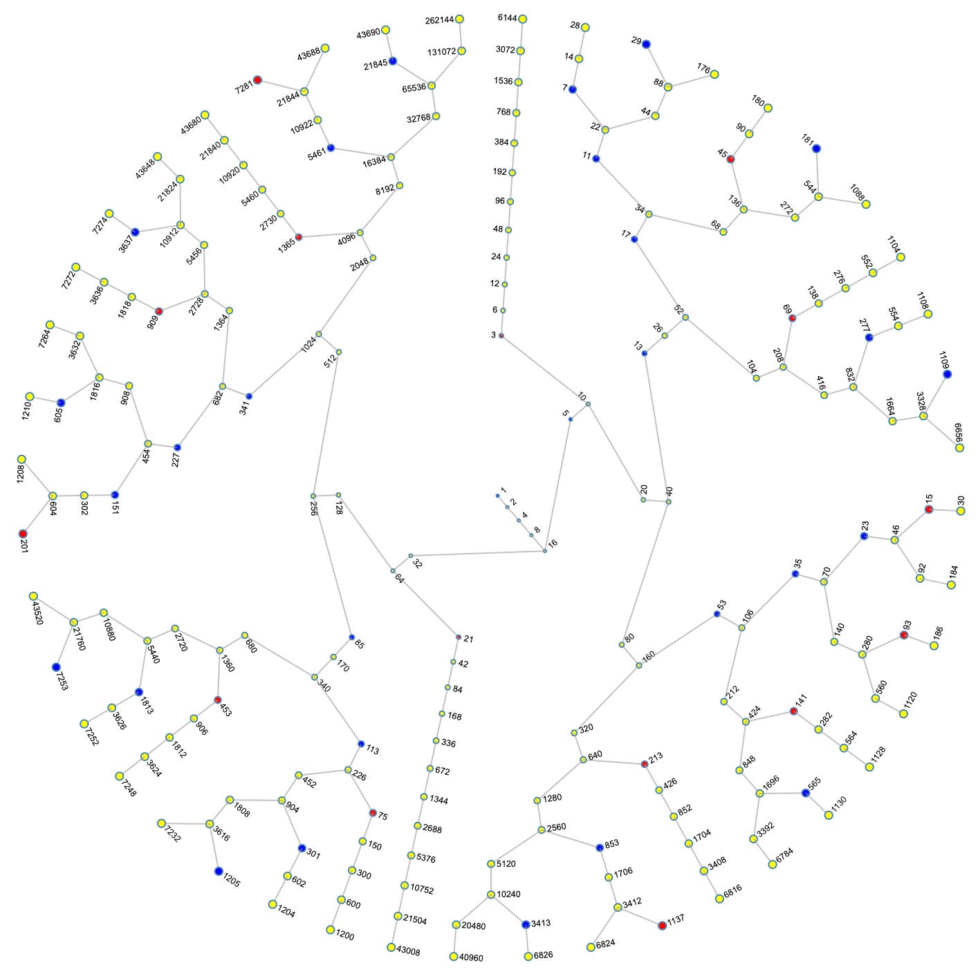
Because the “residue classes” of mod 2 and mod 6 are directly implicated in the generation of the ICM (see Appendix below), it seemed a natural first step to start distinguishing between evens (yellow circles) and odds (red for 3 mod 6, and blue for ±1 mod 6, because that is where all the primes are, and mathematicians always want to know what the primes may, or may not, be up to ;^)). I invite the reader to gaze upon the figure above for a while to see what patterns jump out for you.
A few things I noticed right away was that there are way more even numbers than there are odd numbers, which indicates there are generally a lot more divisions by 2 in the Collatz function than there are multiplications by 3. That in turn would seem to suffice to infer that the Collatz conjecture is probably true, but, alas, not enough to convincingly prove that it is always true. Let’s take a look in mod 6:
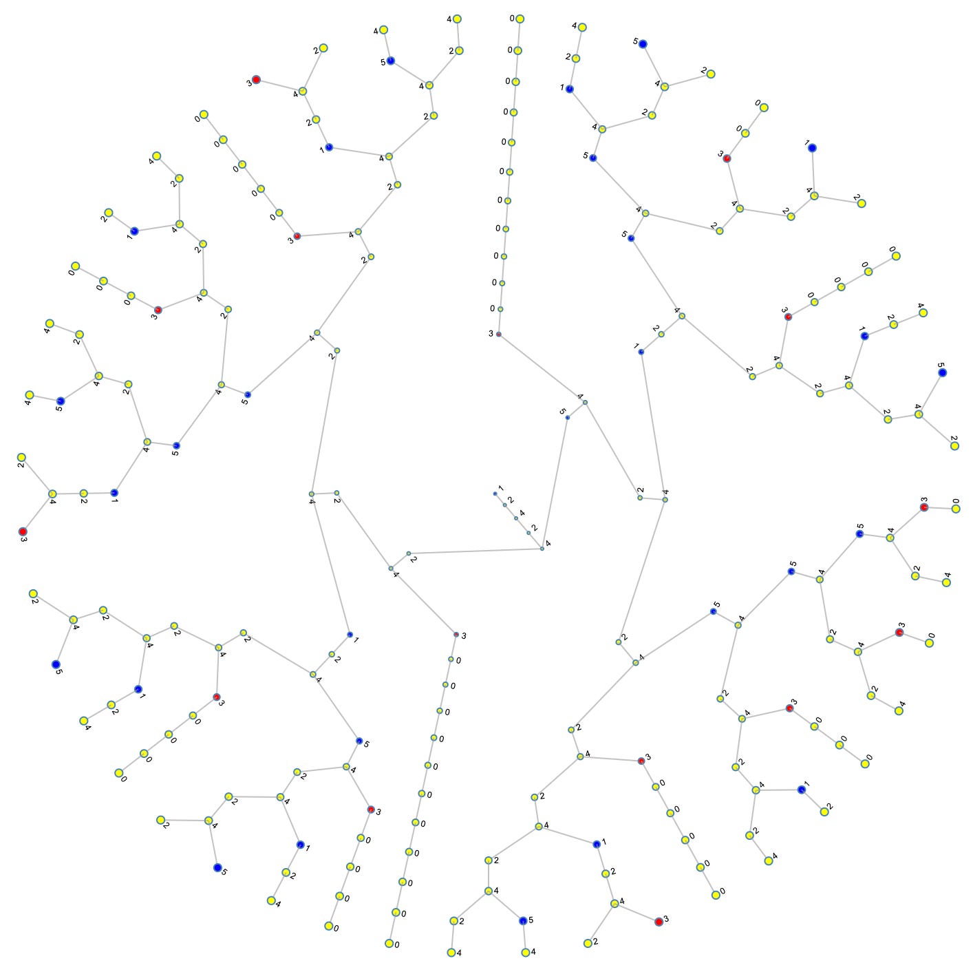
Now things are starting to get much more revealing and much more interesting. Are you starting to feel the affects of the sirens’ seductive song yet? Stay tuned…
APPENDIX: Generating Inverse Collatz Map (ICM)3
Step 1: Initialization
Start at Generation 0 with the number 1:
Step 2: Iterative Construction
To construct generation g from generation g-1, for each number n in generation g-1, generate potential ancestors using two inverse operations:
1. Even Predecessor (always valid):
2. Odd Predecessor (conditionally valid):
Consider the inverse of the operation 3𝑛 + 1:
Include this odd candidate only if both of the following conditions are satisfied:
Hence, the set of numbers in generation g is:
Step 3: Iterate and Continue
Repeat the above iterative process for each subsequent generation as desired.
Explanation of the Odd-Predecessor Criteria
When constructing the ICM, we reverse the Collatz function C(n), defined as:
The even predecessor step is straightforward: to find the predecessor of 𝑛, simply multiply by 2. The odd predecessor step is more subtle and involves careful modular arithmetic considerations. Consider an odd candidate predecessor for a number 𝑛 in generation 𝑔 − 1:
This candidate must satisfy two conditions:
• It must be an integer and odd, as the forward Collatz odd step 3𝑚 + 1 explicitly
originates from an odd number.
• The number 𝑛 at generation 𝑔 − 1 must satisfy 𝑛 ≡ 4 mod 6. This arises from
analyzing the Collatz step modulo 6:
For an odd number m, consider 3m + 1 mod 6:
Thus, the forward operation on an odd number always yields a number congruent to 4 mod 6. To reverse this accurately, we must strictly enforce the modulo 6 criterion.
These two conditions together guarantee that:
• No valid predecessor is missed (completeness).
• No invalid predecessor is erroneously included (correctness).
Hence, each generation 𝑔 accurately and completely enumerates all and only the numbers that are genuinely part of the Inverse Collatz Map structure.
Many thanks to Jason Davies for this mesmorizing simulation of the ICM using Python code by @TerrorBite.
Unlike @TerrorBite, I take 1 as generational level 0, instead of level 1. Guess why…