

Turing Machines
Doubling ones

When I returned to university in the late 1970s to finish my undergraduate studies following a five-year hiatus in the oil and gas industry, I had the good fortune to study logic in an introductory course taught by professor Brian Chellas.1 The text book we were using was Computability and Logic2 by Boolos & Jeffrey. Therein I was introduced to Alan Turing and his Turing machines for the first time, and found them both utterly fascinating.
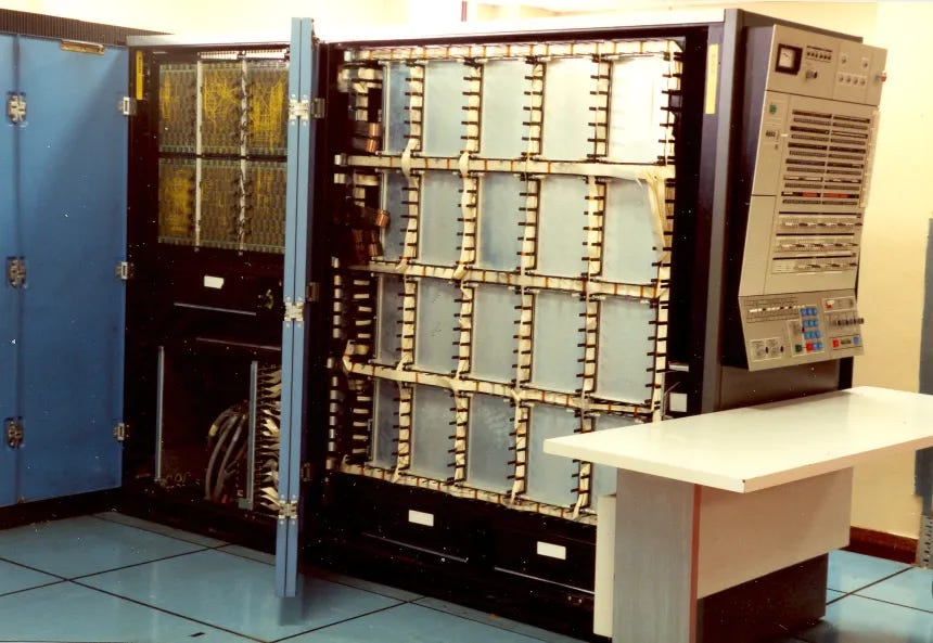
Whilst3 in industry I had the opportunity to operate state-of-the-art mainframe computers for a couple of years, including IBM 360/Series models 44 and 65, which used pre-semiconductor magnetic “core” memory, literally comprised of numerous single bit doughnut-shaped ferrite rings with three criss-crossing wires threaded through them to detect and alter their magnetic states.
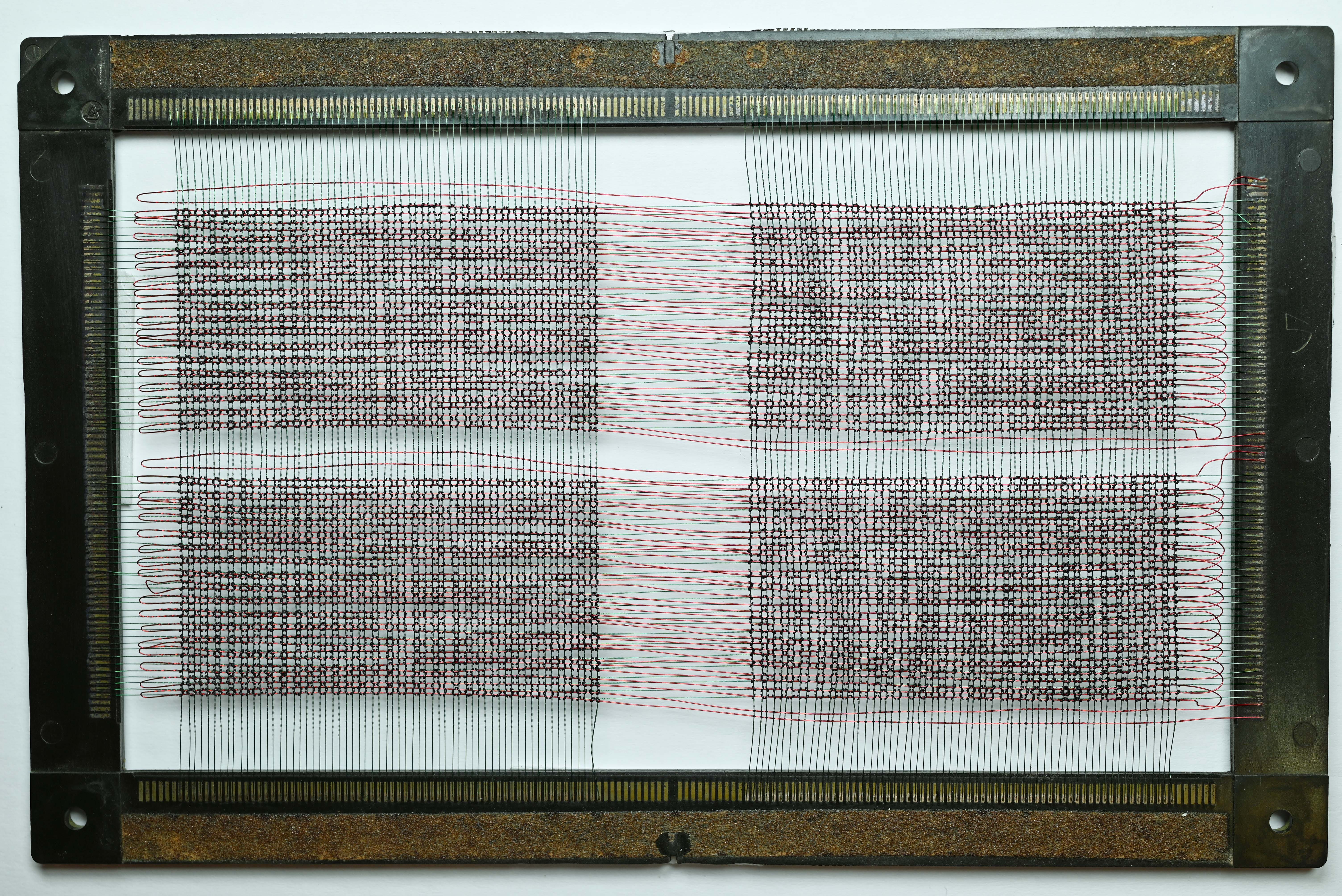
To select a specific core in a grid (a “core plane”), a current was sent through its corresponding X and Y wires. The combined magnetic field at the intersection was strong enough to change the magnetic state of that one core. To read the value of a core, the system would attempt to write a ‘0’ to it. If the core already held a ‘0’, nothing would happen. If it held a ‘1’, the flip in its magnetic state would induce an electrical pulse in a third “sense” wire. Detecting this pulse told the computer that the bit was a ‘1’. Because this process erased the original value, the memory controller then had to rewrite the original value back into the core.
What was so cool about operating these computers was that one could display the contents of specific memory locations using toggle switches on the control panel and write new data directly into core memory. One could, for any given program, literally step through and watch the effect of each individual instruction on the machine’s registers and memory, which were visible on the console’s lights.
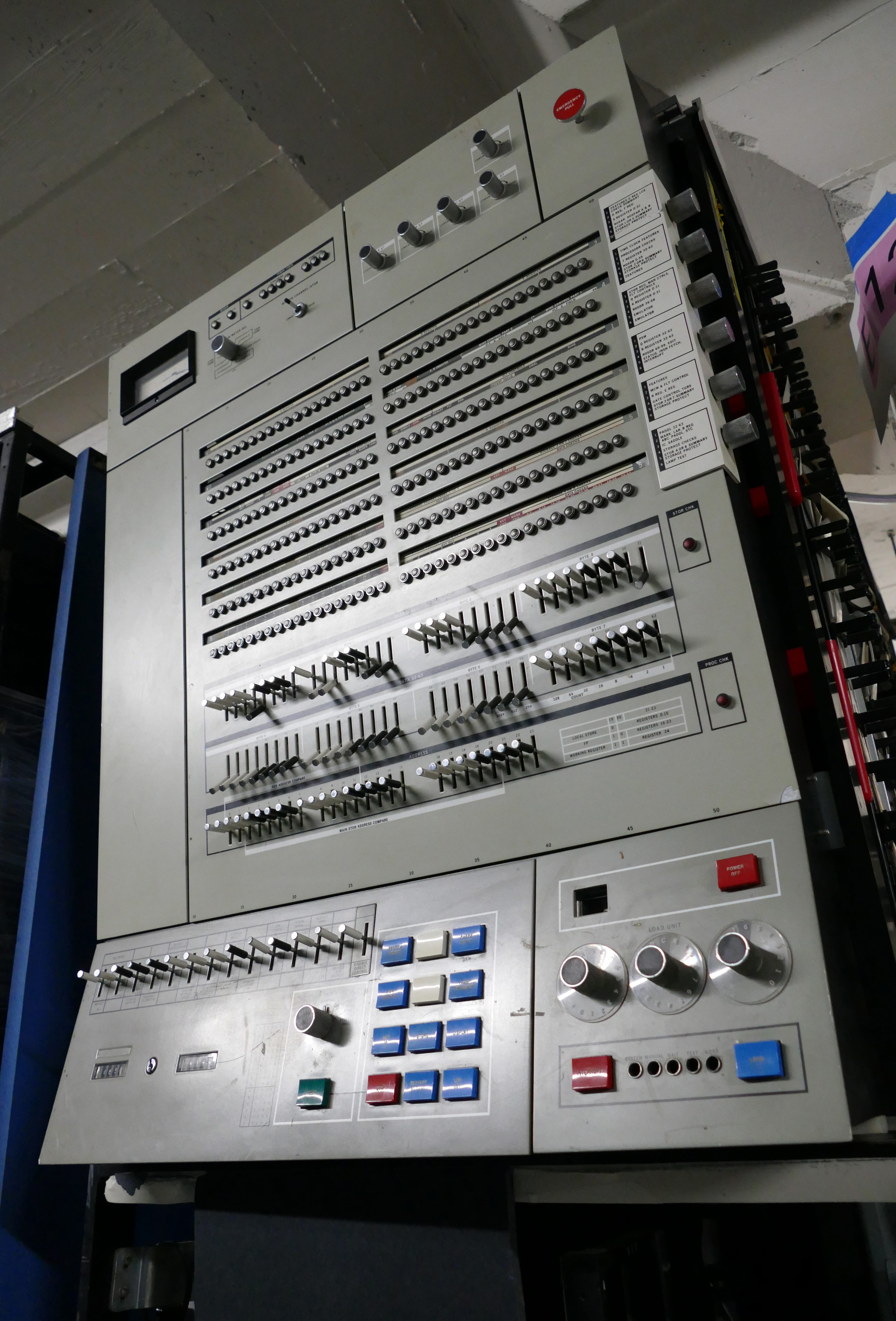
In essence, the control panel switches of the System/360 Model 65 offered a direct, physical connection to the machine’s core memory, allowing for the manual reading, writing, and control of data and instructions that were fundamental to its operation. This level of interaction stands in stark contrast to modern computers, where such low-level access is typically handled by software and no longer exposed through physical controls.
After having operated those iron beasts for a couple of years, being introduced to Turing machines came as a revelation to me that I was well pre-conditioned for. To see the complexity of what those computers were designed and built for reduced to such a simple set of programming instructions I found absolutely captivating.
Alan Turing first conceived of the idea of a universal computing machine in his 1936 paper “On Computable Numbers.”4 Although Turing’s notation in that paper is rather daunting, in essence, a Turing machine consists of three main parts:
An infinitely long tape divided into cells, where each cell holds a single symbol.
A machine head situated on a single cell that can read the symbol in that cell, write a new symbol, and move one step to the left or to the right on the tape.
A finite table of rules that tells the machine head what to do based on its current state and the symbol that it just read.
The machine follows these simple rules to manipulate the symbols on the tape, which is how it performs calculations. Most amazingly, despite its simplicity, a Turing machine is generally taken as capable of simulating the logic of any computer algorithm. The Church-Turing thesis states that if a problem is solvable by a computational method, it is solvable by a Turing machine.
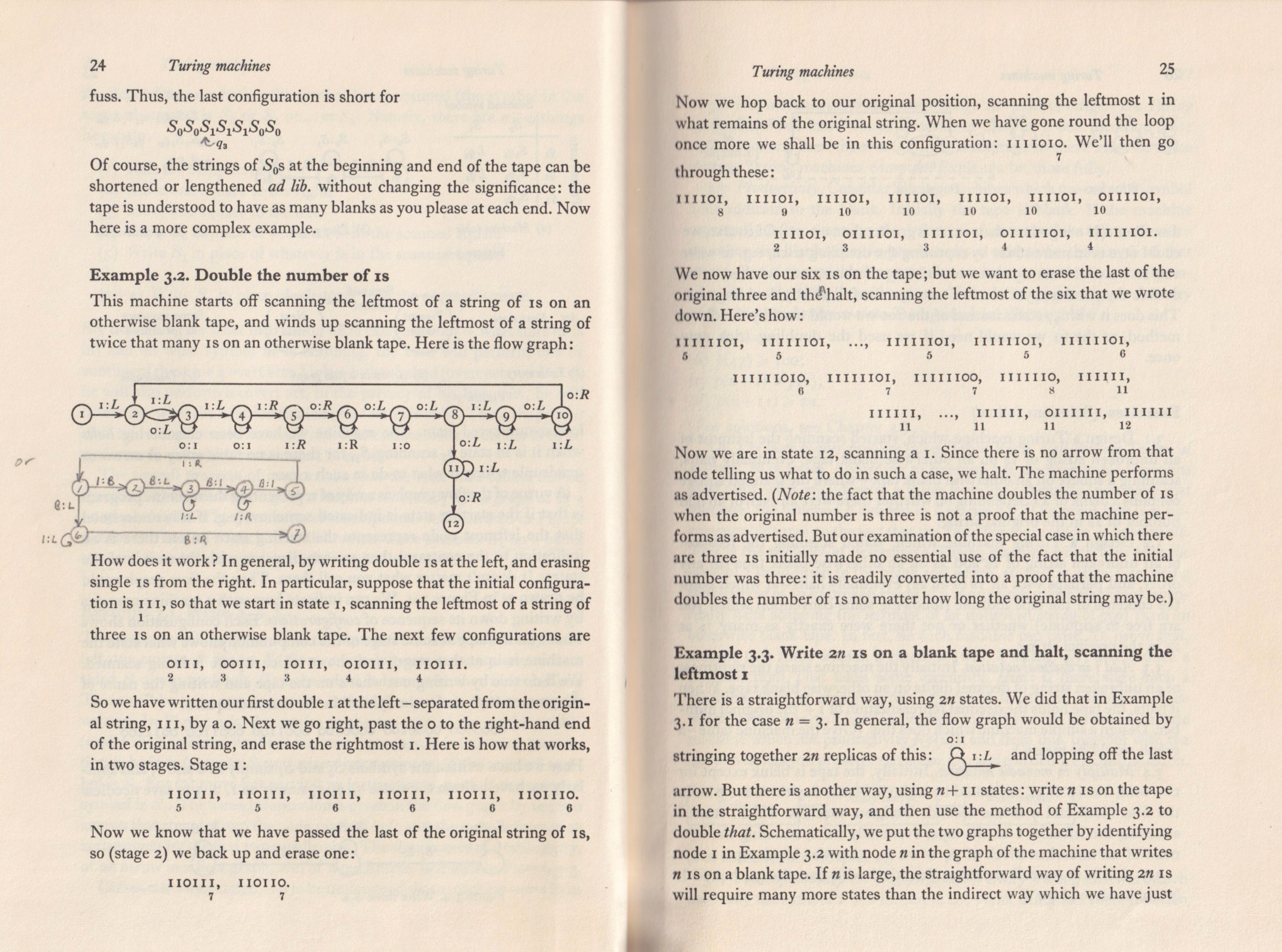
One of the most memorable moments of my undergraduate studies, and the motivation for this post, occurred when professor Chellas demonstrated on the blackboard a 12-State Turing machine designed to double the number of ones on an infinite tape based on this flowchart:
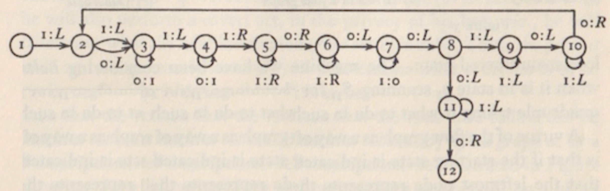
This Turing machine, starting with the first state at the left-most 1 of a string of 1s, reads the 1 and moves one cell to the left (1:L) and enters the second state. It reads the value in that cell, and whether it is a 1 or a 0, it will proceed into the third state (0:L or 1:L). If state 3 is a 0, it will rewrite that cell to contain a 1 (0:1), and if it is a 1 it will move again one cell to the left and enter state 4, etc…
Here is Boolos & Jeffrey’s Turing machine in action, doubling 3 ones:5
I invite the reader to consider whether this algorithm is optimal. I recall that day quite well, because as I watched professor Chellas go through it on the blackboard, my immediate intuitive reaction was that it wasn’t. I was very surprised when he indicated no more optimal algorithm for doubling ones was known.6
I could not get that problem out of my mind, so when I got home I sat down for a couple of hours determined to confirm my intuition that there was a more efficient way of using a Turing machine to double the number of ones. Stop and give it a go yourself if you feel so inclined. If not, continue…
…
…
…
This is what I came up with…
Here, for the sake of comparison, is a speeded up comparison of Booles & Jeffrey’s 12-State Turing machine and my 7-State version, doubling 10 ones:
A couple days later at the beginning of the next class, I told professor Chellas that I had come up with a 7-State Turing machine that doubled the number of ones. I recall it was kind of an awkward moment, which I understand much better now, having taught countless undergraduate courses myself since.
His initial reaction, I could tell, was that I couldn’t possibly have done what I had claimed and this was going to put his pacing off. Bless his heart for having humoured me. Rather than just dismissing my claim and moving along with his lesson plan for the day, he asked for my flow chart, and proceeded to go through it carefully, step-by-step on the blackboard, waiting to uncover whatever error I’m sure he felt sure was there to discover. After going through it once, to his surprise, it worked. Just to be sure, he went through it again to double-check. I’ll never forget his big smile.
He told me he would send my version to his friend and colleague, Richard Jeffrey, which he did. I don’t know if it ever ended up in subsequent editions. Probably not, as it would require a lot of re-writing. Here are the relevant two pages from the text:
Thank goodness I pencilled in my version at the time, otherwise I would have had to figure it out all over again for this post… Thank you, professor Chellas! You did wonders for my confidence.
As for Alan Turing, there is no doubt he was a genius of the first order.
Brian F. Chellas was a Professor Emeritus of Philosophy at the University of Calgary, Canada, where he was affiliated with the Department of Philosophy. He earned his PhD from Stanford University in 1969 with a dissertation titled "The Logical Form of Imperatives". His academic career at the University of Calgary spanned several decades, and he is recognized for his significant contributions to formal philosophy, particularly in the fields of modal logic, deontic logic, and the logic of agency. Professor Chellas passed away March 1, 2023. I humbly dedicate this post to his memory.
Now in its fifth edition! My copy (graciously signed by professor Jeffrey) is the first edition from 1974. How time flies!

;^)
Turing, Alan Mathison. "On computable numbers, with an application to the Entscheidungsproblem." J. of Math 58, no. 345-363 (1936): 5.
Computer program vibe coded with ChatGPT 5 Pro.
I don’t rightly recall if he meant “not known to him,” not known to professor Jeffery, or simply “not known at all.” Whatever the case, it really helped motivate me.